GPU-Accelerated XGBoost with Bayesian Hyperparameter Tuning
Author: Quentin Fournier (edited with LLMs)
This tutorial illustrates a classical machine learning workflow that often serves as a baseline: a GPU-accelerated XGBoost model, combined with Optuna for Bayesian hyperparameter tuning, and SHAP to compute feature importance.
The Full Code is at the end of this guide.
Setting Up the Environment
First, ensure you have the necessary libraries installed.
pip install optuna scikit-learn shap numpy scvi-tools scanpy xgboost optuna-integration[xgboost]
Next, import the necessary modules.
import numpy as np
import matplotlib.pyplot as plt
from sklearn.model_selection import train_test_split

# Dataset
import scvi
import scanpy as sc

# Classifier
import optuna
import xgboost as xgb
import shap

# Display figures in higher quality
%config InlineBackend.figure_format='retina'

# Display Optuna's progress logs.
optuna.logging.set_verbosity(optuna.logging.INFO)
Data Loading and Preprocessing
To demonstrate this workflow on a real-world example, we will use a single-cell RNA sequencing dataset of the human retina, easily accessible through scvi-tools. After loading, we perform standard preprocessing steps: filtering out cells and genes, normalizing the data, log-transforming it, and identifying the most highly variable genes to focus our analysis on. Our goal is to classify the distinct cell types present in the tissue.
print("Loading and preprocessing the retina dataset...")
adata = scvi.data.retina()

# Basic filtering.
sc.pp.filter_cells(adata, min_genes=100)
sc.pp.filter_genes(adata, min_cells=5)
sc.pp.normalize_total(adata, target_sum=1e4)
sc.pp.log1p(adata)
sc.pp.highly_variable_genes(adata)

# Filter for highly variable genes.
adata_filtered = adata[:, adata.var.highly_variable]

# Extract features (X) and labels (y).
X = adata_filtered.X
y = adata_filtered.obs["labels"].cat.codes.to_numpy()
num_classes = len(adata_filtered.obs["labels"].cat.categories)

# Split data into stratified training and testing sets.
X_train, X_test, y_train, y_test = train_test_split(X, y, test_size=0.2, random_state=42, stratify=y)

# Create an optimized DMatrix for efficient GPU training.
dtrain = xgb.DMatrix(X_train, label=y_train)

print(f"Training data shape: {X_train.shape}")
print(f"Number of classes: {num_classes}")
This will produce output similar to the following:
Loading and preprocessing the retina dataset...
Training data shape: (15863, 2830)
Number of classes: 15
GPU-Accelerated Hyperparameter Tuning
The Optuna objective function defines the hyperparameter search space. For this multi-class problem, the objective is 'multi:softprob' and the eval_metric is 'mlogloss'. The study.optimize method runs 100 trials, using cross-validation with early stopping to efficiently find the best parameters on the GPU.
def objective(trial):
    """Defines the evaluation function for Optuna."""

    # Define the hyperparameter search space.
    params = {
        "objective": "multi:softprob",
        "num_class": num_classes,
        "eval_metric": "mlogloss",
        "device": "cuda",

        # Tree booster parameters.
        "max_depth": trial.suggest_int("max_depth", 3, 9),
        "learning_rate": trial.suggest_float("learning_rate", 0.01, 0.3, log=True),
        "gamma": trial.suggest_float("gamma", 0.0, 1.0),
        "min_child_weight": trial.suggest_int("min_child_weight", 1, 10),

        # Sampling parameters to prevent overfitting.
        "subsample": trial.suggest_float("subsample", 0.5, 1.0),
        "colsample_bytree": trial.suggest_float("colsample_bytree", 0.5, 1.0),
    }

    # Run 5-fold cross-validation with early stopping.
    cv_results = xgb.cv(
        params=params,
        dtrain=dtrain,
        nfold=5,
        num_boost_round=100,
        early_stopping_rounds=10,
        as_pandas=True,
    )

    # Store the optimal number of trees.
    trial.set_user_attr("n_estimators", len(cv_results))

    # Return the minimum cross-validated mlogloss score.
    return cv_results["test-mlogloss-mean"].min()

# Create and run the Optuna study.
study = optuna.create_study(direction="minimize")
study.optimize(objective, n_trials=100, n_jobs=1)  # n_jobs=1 for single GPU.
This will produce output similar to the following:
[I 2025-08-16 19:36:51,790] A new study created in memory with name: no-name-819bd9b9-3f40-4231-a982-d3e99ded5775
Training data shape: (15863, 2830)
Number of classes: 15
[I 2025-08-16 19:37:12,843] Trial 0 finished with value: 0.07299848625088005 and parameters: {'max_depth': 5, 'learning_rate': 0.1394797661599296, 'gamma': 0.5517971557725442, 'min_child_weight': 6, 'subsample': 0.9381013535187616, 'colsample_bytree': 0.7518535655183214}. Best is trial 0 with value: 0.07299848625088005.
...
[I 2025-08-16 20:14:45,905] Trial 98 finished with value: 0.3971641684197415 and parameters: {'max_depth': 6, 'learning_rate': 0.021563460451393297, 'gamma': 0.018253635205890156, 'min_child_weight': 3, 'subsample': 0.8831558949846091, 'colsample_bytree': 0.526884411538978}. Best is trial 73 with value: 0.060373317355372345.
[I 2025-08-16 20:15:08,379] Trial 99 finished with value: 0.06601568206806917 and parameters: {'max_depth': 6, 'learning_rate': 0.21484055625232798, 'gamma': 0.043053592221175926, 'min_child_weight': 1, 'subsample': 0.9912736055888298, 'colsample_bytree': 0.5507069815796181}. Best is trial 73 with value: 0.060373317355372345.
Training and Evaluating the Final Model
After optimization, the best hyperparameters are used to train the final XGBClassifier on the full training set. The model’s performance is then evaluated on the held-out test set to ensure its accuracy on unseen data.
# Retrieve the best hyperparameters.
best_params = study.best_params
best_params["n_estimators"] = study.best_trial.user_attrs["n_estimators"]
best_params["objective"] = "multi:softprob"
best_params["num_class"] = num_classes
best_params["device"] = "cpu"

# Print search results.
print("\nBest Hyperparameters:")
for key, value in best_params.items():
    print(f"  {key}: {value}")
print(f"\nBest Cross-Validation Score (Logloss): {study.best_value:.4f}")

# Train the final model with the best parameters.
final_model = xgb.XGBClassifier(**best_params)
final_model.fit(X_train, y_train)

# Evaluate model accuracy on the test set.
accuracy = final_model.score(X_test, y_test)
print(f"Final Score on Test Set (Accuracy): {accuracy:.2%}")
This will produce output similar to the following:
Best Hyperparameters:
  max_depth: 5
  learning_rate: 0.1948886436227877
  gamma: 0.031550344870169104
  min_child_weight: 2
  subsample: 0.6699178548078892
  colsample_bytree: 0.5078011037130629
  n_estimators: 100
  objective: multi:softprob
  num_class: 15
  device: cpu

Best Cross-Validation Score (Logloss): 0.0604
Final Score on Test Set (Accuracy): 98.26%
Visualizing Optimization & Interpretability
Optuna’s built-in plots and SHAP visuals provide insight into the model.
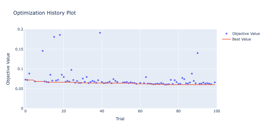
The optimization history plot shows how the objective value improved over each trial.
optuna.visualization.plot_optimization_history(study)

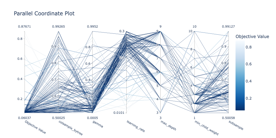
The parallel coordinate plot illustrates the relationship between parameters and the objective value.
optuna.visualization.plot_parallel_coordinate(study)

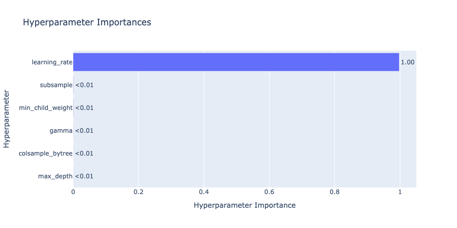
The hyperparameter importances plot quantifies which parameters had the greatest impact on performance.
optuna.visualization.plot_param_importances(study)

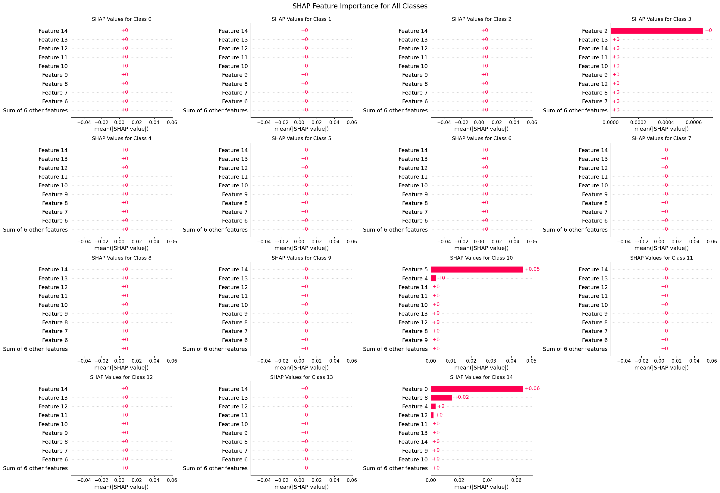
A SHAP explainer is used to understand the model’s predictions. For this multi-class problem, a grid of SHAP bar plots is generated, with each plot showing the most influential genes for a specific cell type.
# Initialize the SHAP explainer.
explainer = shap.TreeExplainer(final_model)

# Calculate SHAP values for the test set.
explanation = explainer(X_test)

# Create a bar plot to visualize global feature importance.
n_cols = int(np.ceil(np.sqrt(num_classes)))
n_rows = int(np.ceil(num_classes / n_cols))
fig, axes = plt.subplots(n_rows, n_cols, figsize=(n_cols * 6, n_rows * 4))
axes = axes.flatten()

for i in range(num_classes):
    shap.plots.bar(explanation[:, i], show=False, ax=axes[i])
    axes[i].set_title(f'SHAP Values for Class {i}', fontsize=12)

# Remove unused subplots.
for j in range(num_classes, len(axes)):
    fig.delaxes(axes[j])

plt.tight_layout()
plt.suptitle('SHAP Feature Importance for All Classes', y=1.02, fontsize=16)
plt.show()

Full Code
Here is all the code from this tutorial in a single block.
import shap
import optuna
import numpy as np
import xgboost as xgb
import scanpy as sc
import scvi
from sklearn.model_selection import train_test_split
import matplotlib.pyplot as plt

# Display Optuna's progress logs.
optuna.logging.set_verbosity(optuna.logging.INFO)

# --- 1. Load and preprocess the retina dataset ---
print("Loading and preprocessing the retina dataset...")
adata = scvi.data.retina()

# Basic filtering.
sc.pp.filter_cells(adata, min_genes=100)
sc.pp.filter_genes(adata, min_cells=5)
sc.pp.normalize_total(adata, target_sum=1e4)
sc.pp.log1p(adata)
sc.pp.highly_variable_genes(adata)

# Filter for highly variable genes.
adata_filtered = adata[:, adata.var.highly_variable]

# Extract features (X) and labels (y).
X = adata_filtered.X
y = adata_filtered.obs["labels"].cat.codes.to_numpy()
num_classes = len(adata_filtered.obs["labels"].cat.categories)

# Split data into stratified training and testing sets.
X_train, X_test, y_train, y_test = train_test_split(X, y, test_size=0.2, random_state=42, stratify=y)

# Create an optimized DMatrix.
dtrain = xgb.DMatrix(X_train, label=y_train)

print(f"Training data shape: {X_train.shape}")
print(f"Number of classes: {num_classes}")


# --- 2. Define and run the Optuna study ---
def objective(trial):
    """Defines the evaluation function for Optuna."""

    # Define the hyperparameter search space.
    params = {
        "objective": "multi:softprob",
        "num_class": num_classes,
        "eval_metric": "mlogloss",
        "device": "cuda",

        # Tree booster parameters.
        "max_depth": trial.suggest_int("max_depth", 3, 9),
        "learning_rate": trial.suggest_float("learning_rate", 0.01, 0.3, log=True),
        "gamma": trial.suggest_float("gamma", 0.0, 1.0),
        "min_child_weight": trial.suggest_int("min_child_weight", 1, 10),

        # Sampling parameters to prevent overfitting.
        "subsample": trial.suggest_float("subsample", 0.5, 1.0),
        "colsample_bytree": trial.suggest_float("colsample_bytree", 0.5, 1.0),
    }

    # Run 5-fold cross-validation with early stopping.
    cv_results = xgb.cv(
        params=params,
        dtrain=dtrain,
        nfold=5,
        num_boost_round=100,
        early_stopping_rounds=10,
        as_pandas=True,
    )

    # Store the optimal number of trees.
    trial.set_user_attr("n_estimators", len(cv_results))

    # Return the minimum cross-validated mlogloss score.
    return cv_results["test-mlogloss-mean"].min()


# Create and run the Optuna study.
study = optuna.create_study(direction="minimize")
study.optimize(objective, n_trials=100, n_jobs=1)

# --- 3. Get best parameters and train final model ---
# Retrieve the best hyperparameters.
best_params = study.best_params
best_params["n_estimators"] = study.best_trial.user_attrs["n_estimators"]
best_params["objective"] = "multi:softprob"
best_params["num_class"] = num_classes
best_params["device"] = "cpu"

# Print search results.
print("\nBest Hyperparameters:")
for key, value in best_params.items():
    print(f"  {key}: {value}")
print(f"\nBest Cross-Validation Score (Logloss): {study.best_value:.4f}")

# Train the final model with the best parameters.
final_model = xgb.XGBClassifier(**best_params)
final_model.fit(X_train, y_train)

# Evaluate model accuracy on the test set.
accuracy = final_model.score(X_test, y_test)
print(f"Final Score on Test Set (Accuracy): {accuracy:.2%}")

# --- Visualize the hyper-parameter search ---
optuna.visualization.plot_optimization_history(study)
optuna.visualization.plot_parallel_coordinate(study)
optuna.visualization.plot_param_importances(study)

# --- 4. Model interpretability with SHAP ---
# Initialize the SHAP explainer.
explainer = shap.TreeExplainer(final_model)

# Calculate SHAP values for the test set.
explanation = explainer(X_test)

# Create a bar plot to visualize global feature importance.
n_cols = int(np.ceil(np.sqrt(num_classes)))
n_rows = int(np.ceil(num_classes / n_cols))
fig, axes = plt.subplots(n_rows, n_cols, figsize=(n_cols * 6, n_rows * 4))
axes = axes.flatten()

for i in range(num_classes):
    shap.plots.bar(explanation[:, i], show=False, ax=axes[i])
    axes[i].set_title(f'SHAP Values for Class {i}', fontsize=12)

# Remove unused subplots.
for j in range(num_classes, len(axes)):
    fig.delaxes(axes[j])

plt.tight_layout()
plt.suptitle('SHAP Feature Importance for All Classes', y=1.02, fontsize=16)
plt.show()